A PEM Survival Model with Time-Dependent Effects
In [4]:
%load_ext autoreload
%autoreload 2
%matplotlib inline
import random
random.seed(13847942484)
import survivalstan
import numpy as np
import pandas as pd
from stancache import stancache
from matplotlib import pyplot as plt
INFO:stancache.seed:Setting seed to 1245502385
The autoreload extension is already loaded. To reload it, use:
  %reload_ext autoreload
In [5]:
print(survivalstan.models.pem_survival_model_timevarying)
/*  Variable naming:
 // dimensions
 N          = total number of observations (length of data)
 S          = number of sample ids
 T          = max timepoint (number of timepoint ids)
 M          = number of covariates

 // data
 s          = sample id for each obs
 t          = timepoint id for each obs
 event      = integer indicating if there was an event at time t for sample s
 x          = matrix of real-valued covariates at time t for sample n [N, X]
 obs_t      = observed end time for interval for timepoint for that obs

*/
// Jacqueline Buros Novik <jackinovik@gmail.com>

functions {
  matrix spline(vector x, int N, int H, vector xi, int P) {
    matrix[N, H + P] b_x;         // expanded predictors
    for (n in 1:N) {
        for (p in 1:P) {
            b_x[n,p] <- pow(x[n],p-1);  // x[n]^(p-1)
        }
        for (h in 1:H)
          b_x[n, h + P] <- fmax(0, pow(x[n] - xi[h],P-1));
    }
    return b_x;
  }
}
data {
  // dimensions
  int<lower=1> N;
  int<lower=1> S;
  int<lower=1> T;
  int<lower=0> M;

  // data matrix
  int<lower=1, upper=N> s[N];     // sample id
  int<lower=1, upper=T> t[N];     // timepoint id
  int<lower=0, upper=1> event[N]; // 1: event, 0:censor
  matrix[N, M] x;                 // explanatory vars

  // timepoint data
  vector<lower=0>[T] t_obs;
  vector<lower=0>[T] t_dur;
}
transformed data {
  vector[T] log_t_dur;
  int n_trans[S, T];

  log_t_dur = log(t_obs);

  // n_trans used to map each sample*timepoint to n (used in gen quantities)
  // map each patient/timepoint combination to n values
  for (n in 1:N) {
      n_trans[s[n], t[n]] = n;
  }

  // fill in missing values with n for max t for that patient
  // ie assume "last observed" state applies forward (may be problematic for TVC)
  // this allows us to predict failure times >= observed survival times
  for (samp in 1:S) {
      int last_value;
      last_value = 0;
      for (tp in 1:T) {
          // manual says ints are initialized to neg values
          // so <=0 is a shorthand for "unassigned"
          if (n_trans[samp, tp] <= 0 && last_value != 0) {
              n_trans[samp, tp] = last_value;
          } else {
              last_value = n_trans[samp, tp];
          }
      }
  }
}
parameters {
  vector[T] log_baseline_raw;    // unstructured baseline hazard for each timepoint t
  real<lower=0> baseline_sigma;
  real log_baseline_mu;

  vector[M] beta; // beta-intercept
  vector<lower=0>[M] beta_time_sigma;
  vector[T-1] raw_beta_time_deltas[M]; // for each coefficient
                                       // change in coefficient value from previous time
}
transformed parameters {
  vector[N] log_hazard;
  vector[T] log_baseline;
  vector[T] beta_time[M];
  vector[T] beta_time_deltas[M];

  // adjust baseline hazard for duration of each period
  log_baseline = log_baseline_raw + log_t_dur;

  // compute timepoint-specific betas
  // offsets from previous time
  for (coef in 1:M) {
      beta_time_deltas[coef][1] = 0;
      for (time in 2:T) {
          beta_time_deltas[coef][time] = raw_beta_time_deltas[coef][time-1];
      }
  }

  // coefficients for each timepoint T
  for (coef in 1:M) {
      beta_time[coef] = beta[coef] + cumulative_sum(beta_time_deltas[coef]);
  }

  // compute log-hazard for each obs
  for (n in 1:N) {
    real log_linpred;
    log_linpred <- 0;
    for (coef in 1:M) {
      // for now, handle each coef separately
      // (to be sure we pull out the "right" beta..)
      log_linpred = log_linpred + x[n, coef] * beta_time[coef][t[n]];
    }
    log_hazard[n] = log_baseline_mu + log_baseline[t[n]] + log_linpred;
  }
}
model {
  // priors on time-varying coefficients
  for (m in 1:M) {
    raw_beta_time_deltas[m][1] ~ normal(0, 100);
    for(i in 2:(T-1)){
        raw_beta_time_deltas[m][i] ~ normal(raw_beta_time_deltas[m][i-1], beta_time_sigma[m]);
    }
  }
  beta_time_sigma ~ cauchy(0, 1);
  beta ~ cauchy(0, 1);

  // priors on baseline hazard
  log_baseline_mu ~ normal(0, 1);
  baseline_sigma ~ normal(0, 1);
  log_baseline_raw[1] ~ normal(0, 1);
  for (i in 2:T) {
      log_baseline_raw[i] ~ normal(log_baseline_raw[i-1], baseline_sigma);
  }

  // model
  event ~ poisson_log(log_hazard);
}
generated quantities {
  real log_lik[N];
  vector[T] baseline;
  int y_hat_mat[S, T];     // ppcheck for each S*T combination
  real y_hat_time[S];      // predicted failure time for each sample
  int y_hat_event[S];      // predicted event (0:censor, 1:event)

  // compute raw baseline hazard, for summary/plotting
  baseline = exp(log_baseline_raw);

  // log_likelihood for loo-psis
  for (n in 1:N) {
      log_lik[n] <- poisson_log_lpmf(event[n] | log_hazard[n]);
  }

  // posterior predicted values
  for (samp in 1:S) {
      int sample_alive;
      sample_alive = 1;
      for (tp in 1:T) {
        if (sample_alive == 1) {
              int n;
              int pred_y;
              real log_linpred;
              real log_haz;

              // determine predicted value of y
              n = n_trans[samp, tp];

              // (borrow code from above to calc linpred)
              // but use sim tp not t[n]
              log_linpred = 0;
              for (coef in 1:M) {
                  // for now, handle each coef separately
                  // (to be sure we pull out the "right" beta..)
                  log_linpred = log_linpred + x[n, coef] * beta_time[coef][tp];
              }
              log_haz = log_baseline_mu + log_baseline[tp] + log_linpred;

              // now, make posterior prediction
              if (log_haz < log(pow(2, 30)))
                  pred_y = poisson_log_rng(log_haz);
              else
                  pred_y = 9;

              // mark this patient as ineligible for future tps
              // note: deliberately make 9s ineligible
              if (pred_y >= 1) {
                  sample_alive = 0;
                  y_hat_time[samp] = t_obs[tp];
                  y_hat_event[samp] = 1;
              }

              // save predicted value of y to matrix
              y_hat_mat[samp, tp] = pred_y;
          }
          else if (sample_alive == 0) {
              y_hat_mat[samp, tp] = 9;
          }
      } // end per-timepoint loop

      // if patient still alive at max
      //
      if (sample_alive == 1) {
          y_hat_time[samp] = t_obs[T];
          y_hat_event[samp] = 0;
      }
  } // end per-sample loop
}
In [6]:
d = stancache.cached(
    survivalstan.sim.sim_data_exp_correlated,
    N=100,
    censor_time=20,
    rate_form='1 + sex',
    rate_coefs=[-3, 0.5],
)
d['age_centered'] = d['age'] - d['age'].mean()
d.head()
INFO:stancache.stancache:sim_data_exp_correlated: cache_filename set to sim_data_exp_correlated.cached.N_100.censor_time_20.rate_coefs_54462717316.rate_form_1 + sex.pkl
INFO:stancache.stancache:sim_data_exp_correlated: Loading result from cache
Out[6]:
| age | sex | rate | true_t | t | event | index | age_centered | |
|---|---|---|---|---|---|---|---|---|
| 0 | 59 | male | 0.082085 | 20.948771 | 20.000000 | False | 0 | 4.18 |
| 1 | 58 | male | 0.082085 | 12.827519 | 12.827519 | True | 1 | 3.18 |
| 2 | 61 | female | 0.049787 | 27.018886 | 20.000000 | False | 2 | 6.18 |
| 3 | 57 | female | 0.049787 | 62.220296 | 20.000000 | False | 3 | 2.18 |
| 4 | 55 | male | 0.082085 | 10.462045 | 10.462045 | True | 4 | 0.18 |
In [7]:
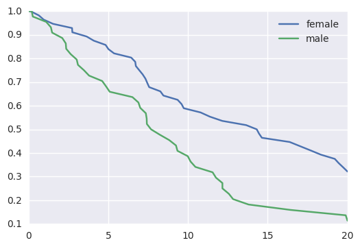
survivalstan.utils.plot_observed_survival(df=d[d['sex']=='female'], event_col='event', time_col='t', label='female')
survivalstan.utils.plot_observed_survival(df=d[d['sex']=='male'], event_col='event', time_col='t', label='male')
plt.legend()
Out[7]:
<matplotlib.legend.Legend at 0x7f6f245cc550>
In [8]:
dlong = stancache.cached(
    survivalstan.prep_data_long_surv,
    df=d, event_col='event', time_col='t'
)
dlong.sort_values(['index', 'end_time'], inplace=True)
INFO:stancache.stancache:prep_data_long_surv: cache_filename set to prep_data_long_surv.cached.df_33772694934.event_col_event.time_col_t.pkl
INFO:stancache.stancache:prep_data_long_surv: Loading result from cache
In [9]:
dlong.head()
Out[9]:
| age | sex | rate | true_t | t | event | index | age_centered | key | end_time | end_failure | |
|---|---|---|---|---|---|---|---|---|---|---|---|
| 62 | 59 | male | 0.082085 | 20.948771 | 20.0 | False | 0 | 4.18 | 1 | 0.118611 | False |
| 3 | 59 | male | 0.082085 | 20.948771 | 20.0 | False | 0 | 4.18 | 1 | 0.196923 | False |
| 61 | 59 | male | 0.082085 | 20.948771 | 20.0 | False | 0 | 4.18 | 1 | 0.262114 | False |
| 71 | 59 | male | 0.082085 | 20.948771 | 20.0 | False | 0 | 4.18 | 1 | 0.641174 | False |
| 26 | 59 | male | 0.082085 | 20.948771 | 20.0 | False | 0 | 4.18 | 1 | 0.944220 | False |
In [10]:
testfit = survivalstan.fit_stan_survival_model(
    model_cohort = 'test model',
    model_code = survivalstan.models.pem_survival_model_timevarying,
    df = dlong,
    sample_col = 'index',
    timepoint_end_col = 'end_time',
    event_col = 'end_failure',
    formula = '~ age_centered + sex',
    iter = 10000,
    chains = 4,
    seed = 9001,
    FIT_FUN = stancache.cached_stan_fit,
    )
INFO:stancache.stancache:Step 1: Get compiled model code, possibly from cache
INFO:stancache.stancache:StanModel: cache_filename set to anon_model.cython_0_25_1.model_code_9304163442804524267.pystan_2_12_0_0.stanmodel.pkl
INFO:stancache.stancache:StanModel: Loading result from cache
INFO:stancache.stancache:Step 2: Get posterior draws from model, possibly from cache
INFO:stancache.stancache:sampling: cache_filename set to anon_model.cython_0_25_1.model_code_9304163442804524267.pystan_2_12_0_0.stanfit.chains_4.data_75232070308.iter_10000.seed_9001.pkl
INFO:stancache.stancache:sampling: Loading result from cache
/home/jacquelineburos/miniconda3/envs/python3/lib/python3.5/site-packages/stanity/psis.py:228: FutureWarning: elementwise comparison failed; returning scalar instead, but in the future will perform elementwise comparison
  elif sort == 'in-place':
/home/jacquelineburos/miniconda3/envs/python3/lib/python3.5/site-packages/stanity/psis.py:246: VisibleDeprecationWarning: using a non-integer number instead of an integer will result in an error in the future
  bs /= 3 * x[sort[np.floor(n/4 + 0.5) - 1]]
/home/jacquelineburos/miniconda3/envs/python3/lib/python3.5/site-packages/stanity/psis.py:262: RuntimeWarning: overflow encountered in exp
  np.exp(temp, out=temp)
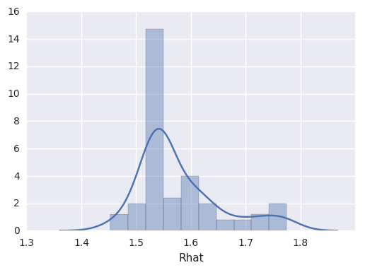
superficial check of convergence
In [11]:
survivalstan.utils.print_stan_summary([testfit], pars='lp__')
            mean    se_mean          sd        2.5%         50%       97.5%      Rhat
lp__  407.328012  15.738683  101.998321  214.786192  407.532163  606.393469  1.059665
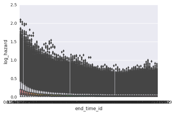
In [12]:
survivalstan.utils.plot_stan_summary([testfit], pars='log_baseline')
summarize coefficient estimates
In [13]:
survivalstan.utils.plot_coefs([testfit], element='baseline')
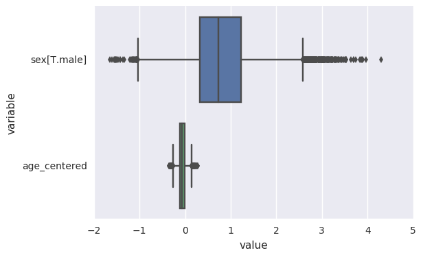
In [14]:
survivalstan.utils.plot_coefs([testfit])
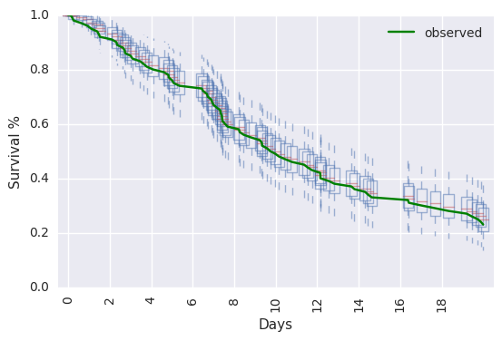
posterior-predictive checks
In [15]:
survivalstan.utils.plot_pp_survival([testfit], fill=False)
survivalstan.utils.plot_observed_survival(df=d, event_col='event', time_col='t', color='green', label='observed')
plt.legend()
Out[15]:
<matplotlib.legend.Legend at 0x7f6f0407b630>
In [16]:
survivalstan.utils.plot_pp_survival([testfit], by='sex')
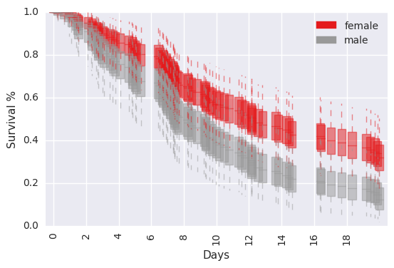
In [23]:
survivalstan.utils.plot_pp_survival([testfit], by='sex', pal=['red', 'blue'])
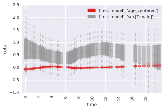
summarize time-varying effect of sex on survival
Standard behavior is to plot estimated betas at each timepoint, for each coefficient in the model.
In [31]:
survivalstan.utils.plot_coefs([testfit], element='beta_time', ylim=[-1, 2.5])
accessing lower-level functions for plotting effects over time
In [26]:
survivalstan.utils.plot_time_betas(models=[testfit], by=['coef'], y='exp(beta)', ylim=[0, 10])
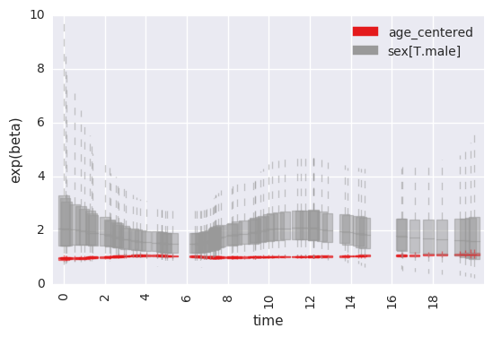
Alternatively, you can extract the beta-estimates for each timepoint & plot them yourself.
In [27]:
testfit['time_beta'] = survivalstan.utils.extract_time_betas([testfit])
testfit['time_beta'].head()
Out[27]:
| timepoint_id | beta | coef | end_time | exp(beta) | model_cohort | |
|---|---|---|---|---|---|---|
| 0 | 1 | 0.281855 | sex[T.male] | 0.118611 | 1.325587 | test model |
| 1 | 1 | 1.263018 | sex[T.male] | 0.118611 | 3.536076 | test model |
| 2 | 1 | 0.875265 | sex[T.male] | 0.118611 | 2.399512 | test model |
| 3 | 1 | 0.128097 | sex[T.male] | 0.118611 | 1.136664 | test model |
| 4 | 1 | 0.185878 | sex[T.male] | 0.118611 | 1.204276 | test model |
You can also extract and/or plot data for single coefficients of interest at a time.
In [28]:
first_beta = survivalstan.utils.extract_time_betas([testfit], coefs=['sex[T.male]'])
first_beta.head()
Out[28]:
| timepoint_id | beta | coef | end_time | exp(beta) | model_cohort | |
|---|---|---|---|---|---|---|
| 0 | 1 | 0.281855 | sex[T.male] | 0.118611 | 1.325587 | test model |
| 1 | 1 | 1.263018 | sex[T.male] | 0.118611 | 3.536076 | test model |
| 2 | 1 | 0.875265 | sex[T.male] | 0.118611 | 2.399512 | test model |
| 3 | 1 | 0.128097 | sex[T.male] | 0.118611 | 1.136664 | test model |
| 4 | 1 | 0.185878 | sex[T.male] | 0.118611 | 1.204276 | test model |
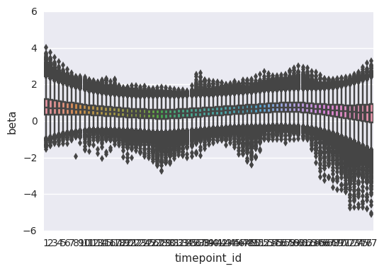
In [30]:
import seaborn as sns
sns.boxplot(data=first_beta, x='timepoint_id', y='beta')
Out[30]:
<matplotlib.axes._subplots.AxesSubplot at 0x7f6f0d2f3518>
In [32]:
survivalstan.utils.plot_time_betas(models=[testfit], y='beta', x='end_time', coefs=['sex[T.male]'])
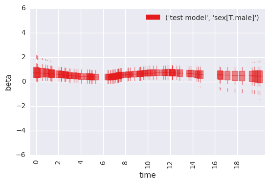
Note that this same plot can be produced by passing data to
plot_time_betas directly.
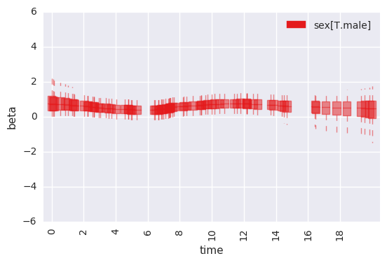
In [33]:
survivalstan.utils.plot_time_betas(df=first_beta, by=['coef'], y='beta', x='end_time')
In [ ]: